While the expected-utility model includes a straightforward decision rule, it does not include a method for calculating pivot probabilities. Indeed this calculation appears to be anything but straightforward. Several approaches to this calculation from the literature are presented and analyzed here. These approaches all become more computationally complex as the number of election alternatives increases. We introduce a novel approach that does not increase in complexity with the number alternatives.
Before discussing methods for calculating pivot probabilities, it is
useful to examine the definition of pivot probability in more detail.
As already mentioned, a voter's pivot probability for any two
candidates is the probability that he or she will be decisive in
making or breaking an ![]() -place tie between those two
candidates. If we assume that for each possible election outcome we
can determine the probability associated with the occurrence of that
outcome, the pivot probability is the sum of the probabilities
associated with each of the possible election outcomes that involve an
-place tie between those two
candidates. If we assume that for each possible election outcome we
can determine the probability associated with the occurrence of that
outcome, the pivot probability is the sum of the probabilities
associated with each of the possible election outcomes that involve an
![]() -place tie between those two candidates.
-place tie between those two candidates.
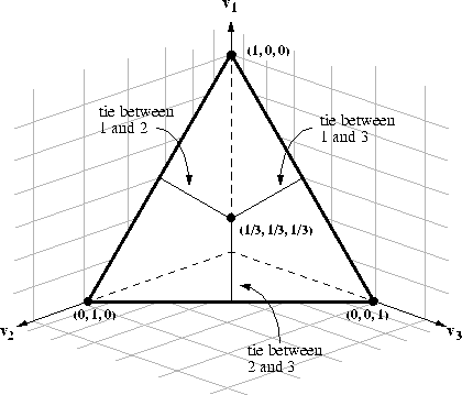
Figure: A three-dimensional view of the barycentric coordinate system
The election outcome space for a three-candidate election can be
represented visually as a barycentric coordinate system -- an
equilateral triangle on the three-dimensional plane ![]() , where
, where ![]() ,
, ![]() , and
, and ![]() represent the
proportions of votes for candidates 1, 2, and 3 respectively.
Each of the triangle corners represents one candidate. The closer an
outcome point is to a particular corner, the more votes the
alternative represented by that corner received. Thus, an outcome
point in a corner of the triangle represents a ``shut-out'' in which
one alternative received all the votes, while an outcome point in the
geometrical center of the triangle represents a three-way tie. As
shown in Figure
represent the
proportions of votes for candidates 1, 2, and 3 respectively.
Each of the triangle corners represents one candidate. The closer an
outcome point is to a particular corner, the more votes the
alternative represented by that corner received. Thus, an outcome
point in a corner of the triangle represents a ``shut-out'' in which
one alternative received all the votes, while an outcome point in the
geometrical center of the triangle represents a three-way tie. As
shown in Figure ![]() , the line segments that bisect the
triangle represent two-way winning ties. This model can be extended
arbitrarily. For an election with four alternatives the barycentric
triangle becomes a solid tetrahedron. An election with N
alternatives can be represented by a simplex polyhedron of N - 1
dimensions.
, the line segments that bisect the
triangle represent two-way winning ties. This model can be extended
arbitrarily. For an election with four alternatives the barycentric
triangle becomes a solid tetrahedron. An election with N
alternatives can be represented by a simplex polyhedron of N - 1
dimensions.
Because finding the candidate that maximizes the expected-gain equations (Equation 1) depends on the ratio of the pivot probabilities rather than the actual probabilities themselves, we do not need to find a method for calculating the absolute probability of reaching each point in the outcome space; rather, it is sufficient to find a method of calculating relative probabilities. Thus the methods we examine here do not necessarily result in the probabilities over the entire outcome space summing to 1.
When comparing probability calculation methods and analyzing the
suitable of each for use in the expected-utility model of voting, it
is helpful to be able to visualize the behavior of the
expected-utility model when different probability calculation methods
are used. Hoffman [55] includes contour plots in his
paper to help illustrate this behavior. To allow visual comparison of
our new method with Hoffman's we wrote a computer program to generate
contour plots such as the one shown in Figure ![]() . The
curves on these plots represent predicted outcome-proportions for a
voter's first choice,
. The
curves on these plots represent predicted outcome-proportions for a
voter's first choice, ![]() , in a three-candidate election.
Predicted outcome-proportions for a voter's second choice,
, in a three-candidate election.
Predicted outcome-proportions for a voter's second choice, ![]() ,
are shown along the x-axis.
,
are shown along the x-axis. ![]() , a voter's utility rating for
, a voter's utility rating for
![]() is shown along the y-axis. Given a predicted outcome at
point
is shown along the y-axis. Given a predicted outcome at
point ![]() , a voter should vote for for
, a voter should vote for for ![]() if and only if the point
if and only if the point ![]() lies above the curve for
outcome
lies above the curve for
outcome ![]() ; otherwise the voter should vote for
; otherwise the voter should vote for ![]() .
Consider, for example a predicted outcome of P = (.15, .4, .45).
Voters who rate
.
Consider, for example a predicted outcome of P = (.15, .4, .45).
Voters who rate ![]() should vote for
should vote for ![]() ; voters
who rate
; voters
who rate ![]() should vote for
should vote for ![]() . The plots
shown in this chapter all assume normalized ratings such that
. The plots
shown in this chapter all assume normalized ratings such that ![]() .
.
We now consider several methods for calculating pivot probabilities.
One approach to calculating pivot probabilities involves making a prediction about the likely outcome of the election, plotting that outcome as a point on a barycentric coordinate system, and computing the relative distances between that outcome point and the outcome lines for each of the two-way ties. Black [14] used this method in a model of a three-candidate plurality election in which each voter was assumed to be able to make a reasonable prediction about the election outcome based on the results of previous elections, opinion polls, or other data. In batched DSV we can determine the voters' sincere strategies from their utility information, and aggregate these strategies to determine a first-round predicted outcome. Subsequent rounds can use the results of the previous round as a predicted outcome. In ballot-by-ballot DSV, the interim tally of ballots counted so far can serve as the predicted outcome point.
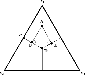
Figure: Distances used to calculate Black's probability estimates
Black assumes that the pivot probability for any pair of candidates is
proportional to 1-d, where d is the Euclidean distance between the
line segment ![]() representing an
representing an ![]() -place tie
between those candidates and the predicted outcome point A, as shown
in Figure
-place tie
between those candidates and the predicted outcome point A, as shown
in Figure ![]() .
.![]() For
For ![]() this distance
this distance ![]() is equivalent to the
length of the perpendicular line segment
is equivalent to the
length of the perpendicular line segment ![]() from the
predicted outcome point to the first-place tie line
from the
predicted outcome point to the first-place tie line ![]() .
.
The distance calculation
for ![]() can be expressed as:
can be expressed as:
![]()
where ![]() and
and ![]() .
The other pivot probabilities can be calculated in a similar manner.
.
The other pivot probabilities can be calculated in a similar manner.
We developed and experimented with a variation on Black's method involves calculating the distance d between the predicted outcome and a given point on a two way tie line. Using this technique, the pivot probability for any two candidates can be found by summing the differences 1-d for every point on the two-way tie line for those candidates. This method makes more intuitive sense than Black's method if one considers what the pivot probabilities really represent.
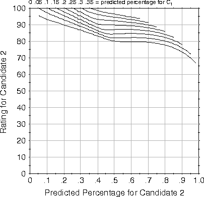
Figure: Contour plot for 3-candidate plurality election using our
simple distance pivot probabilities
One problem with both Black's method and our variation is that
they assume that the probability of a tie gets linearly larger the
farther away a predicted outcome point is from a two-way tie line.
This uniform probability distribution, while simple, does not seem
consistent with empirical evidence. For example, as
Figure ![]() illustrates, these methods rarely select
the strategy of voting for a second-choice candidate unless the
second-choice candidate has a utility rating at least 80% as high as
the first-choice candidate. In addition, these methods do not take
into consideration the certainty of the predicted outcome point.
illustrates, these methods rarely select
the strategy of voting for a second-choice candidate unless the
second-choice candidate has a utility rating at least 80% as high as
the first-choice candidate. In addition, these methods do not take
into consideration the certainty of the predicted outcome point.
Hoffman [55] offers another approach that allows for the
modeling of voting schemes other than simple plurality, and assumes a
Gaussian distribution of outcomes rather than a uniform distribution.
Although Hoffman introduces his approach by describing a
three-candidate election, the approach may be applied to elections
involving any number of candidates and is most easily understood by
considering a two-candidate election first. A two-candidate election
with B voters can be modeled as a line segment. This line segment
can be divided into B smaller segments, each one vote wide, as shown
in Figure ![]() . Each of the smaller line segments represents
a possible election outcome. If there are an odd number of voters,
there will be a line segment T at the center of the line that
represents a tie. If we randomly sample the voters, we can predict an
election outcome and represent it somewhere along our line at segment
P.
. Each of the smaller line segments represents
a possible election outcome. If there are an odd number of voters,
there will be a line segment T at the center of the line that
represents a tie. If we randomly sample the voters, we can predict an
election outcome and represent it somewhere along our line at segment
P.

Figure: Gaussian geometry for a 2-candidate election
Given P, we are interested in determining the probability that the
election outcome will be a tie. As Figure ![]() illustrates,
we can construct a normal distribution curve around the center point of
P, given by the formula
illustrates,
we can construct a normal distribution curve around the center point of
P, given by the formula
![]()
where D is the distance from each point to (the center of) P, and
![]() is a measure of the uncertainty of the prediction. Hoffman does
not specify how
is a measure of the uncertainty of the prediction. Hoffman does
not specify how ![]() should be calculated, but the ``standard error
of the estimate'' seems to be an appropriate measure of uncertainty.
As we shall see,
should be calculated, but the ``standard error
of the estimate'' seems to be an appropriate measure of uncertainty.
As we shall see, ![]() is an important factor and can affect the
outcome of a DSV election dramatically. When using the standard error
to calculate
is an important factor and can affect the
outcome of a DSV election dramatically. When using the standard error
to calculate ![]() in a ballot-by-ballot DSV system, we multiply it by
the finite-population correction factor yielding:
in a ballot-by-ballot DSV system, we multiply it by
the finite-population correction factor yielding:
where ![]() and
and ![]() represent the proportion of votes for each
candidate thus far, B represents the total voter population, b
represents the number of votes counted thus far, and
represent the proportion of votes for each
candidate thus far, B represents the total voter population, b
represents the number of votes counted thus far, and ![]() represents the area under the standard normal curve for confidence
level
represents the area under the standard normal curve for confidence
level ![]() . Thus as the election progresses, b will
increase and
. Thus as the election progresses, b will
increase and ![]() will decrease. The fact that uncertainty
decreases as the election progresses is consistent with the fact that
the amount of information increases.
will decrease. The fact that uncertainty
decreases as the election progresses is consistent with the fact that
the amount of information increases.
The above method of calculating uncertainty is useful for ballot-by-ballot DSV, in which the predicted outcome involves a sample that increases in size until it equals the entire population; however, in batch DSV, the predicted outcome point is based on polling the entire population -- thus our prediction derives no uncertainty from sampling error. In batch DSV the uncertainty of the prediction is based on not knowing how many voters will find that their optimal strategies are not their sincere strategies.
The simplest way to account for uncertainty in batch DSV would be to
select an arbitrary value for ![]() . For example,
. For example, ![]() has the property that as long as a
has the property that as long as a ![]() is predicted to receive at
least 5% of the vote, voters will not vote for
is predicted to receive at
least 5% of the vote, voters will not vote for ![]() unless
unless ![]() is at least 10% as large as
is at least 10% as large as ![]() (on a 10 point scale, a voter
with
(on a 10 point scale, a voter
with ![]() must have
must have ![]() in order to vote for
in order to vote for
![]() ). We used this approach in our simulations, described in
Chapter
). We used this approach in our simulations, described in
Chapter ![]() . We also tried conducting batch DSV
simulations with the number of rounds equal to the number of voters
and adjusting
. We also tried conducting batch DSV
simulations with the number of rounds equal to the number of voters
and adjusting ![]() according to Equation
according to Equation ![]() , letting b
equal the number of rounds run so far. However this approach
generally resulted in the same election outcome as was produced using
a constant
, letting b
equal the number of rounds run so far. However this approach
generally resulted in the same election outcome as was produced using
a constant ![]() equal to the value produced by Equation
equal to the value produced by Equation ![]() when b = B.
when b = B.
Another approach to calculating ![]() would be to develop a formula
based on some aggregation of the utilities submitted by the
voters -- perhaps taking into account the percentage of voters for
whom it might never be optimal to voter for
would be to develop a formula
based on some aggregation of the utilities submitted by the
voters -- perhaps taking into account the percentage of voters for
whom it might never be optimal to voter for ![]() . Such a
calculation is also likely to be somewhat arbitrary, however. Still
another approach would be to assign random values to
. Such a
calculation is also likely to be somewhat arbitrary, however. Still
another approach would be to assign random values to ![]() within a
reasonable range (say .001 - .5). Finally, voters could select
their own uncertainty values based on their attitudes toward risk,
formulated perhaps as a function of the ``maturity'' of the election:
number of rounds, position in the voting sequence, etc.
within a
reasonable range (say .001 - .5). Finally, voters could select
their own uncertainty values based on their attitudes toward risk,
formulated perhaps as a function of the ``maturity'' of the election:
number of rounds, position in the voting sequence, etc.
Regardless of what method is used to calculate ![]() , the
probability that the election outcome will involve a first-place tie
between candidates 1 and 2 can be computed as follows:
, the
probability that the election outcome will involve a first-place tie
between candidates 1 and 2 can be computed as follows:
![]()
where U = 1/B (the length of a one-vote wide line segment). That is, the probability of a tie is proportional to the area under the segment of the normal curve that lies above the tie segment T.
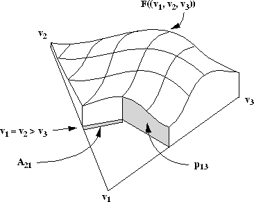
Figure: Hoffman's geometry for a 3-candidate election
Hoffman illustrates his approach for a three-candidate election. As
shown in Figure ![]() , Hoffman specifies the region
, Hoffman specifies the region
![]() as the portion of the outcome triangle in which candidate i
loses to candidate j by one vote (or less in systems that allow
fractional votes). He defines the pivot probability as ``the
probability that the election result
as the portion of the outcome triangle in which candidate i
loses to candidate j by one vote (or less in systems that allow
fractional votes). He defines the pivot probability as ``the
probability that the election result ![]() lies in
the region
lies in
the region ![]() .'' Thus
.'' Thus ![]() can be expressed as:
can be expressed as:
![]()
where D is the distance from the predicted outcome point to a point in
the region ![]() . Because
. Because ![]() is only one vote wide,
is only one vote wide, ![]() can be approximated by using Simpson's rule or another numerical
integration technique to integrate over the outcome points for which
can be approximated by using Simpson's rule or another numerical
integration technique to integrate over the outcome points for which
![]() . Irrespective of the number of candidates
N, first-place ties can occur only when
. Irrespective of the number of candidates
N, first-place ties can occur only when ![]() . Values of
. Values of ![]() and
and ![]() greater than 1/2 would be
impossible because
greater than 1/2 would be
impossible because ![]() ; and values of
; and values of ![]() and
and
![]() less than 1/N would indicate that at least one other
candidate has a higher proportion of the vote. Values of
less than 1/N would indicate that at least one other
candidate has a higher proportion of the vote. Values of ![]() and
and
![]() between 1/N and 1/3 may or may not indicate first-place
ties, depending on the outcome proportions for the other candidates.
However, when
between 1/N and 1/3 may or may not indicate first-place
ties, depending on the outcome proportions for the other candidates.
However, when ![]() ,
, ![]() and
and ![]() must be in a first-place tie. Thus, for a three-candidate election,
must be in a first-place tie. Thus, for a three-candidate election,
![]() can be approximated by:
can be approximated by:
![]()
where x represents the proportion of votes for candidates i and
j at a given outcome point. Note that when N > 2, the standard
error of the estimate becomes quite difficult to calculate. We
use the approximation![]()
to calculate the standard error of the estimate for N > 2.
A four-candidate election is modeled as a solid tetrahedron. However,
finding the outcome region in which first-place ties occur is not as
easy in four dimensions as it is in two and three. As discussed
above, first-place ties may occur in regions where ![]() , depending on the proportion of votes received by each
of the other candidates. With four candidates, the outcome region in
which candidates i and j tie for first place is a kite-shaped
section of the plane. The probability of an outcome occurring in this
region can be approximated by:
, depending on the proportion of votes received by each
of the other candidates. With four candidates, the outcome region in
which candidates i and j tie for first place is a kite-shaped
section of the plane. The probability of an outcome occurring in this
region can be approximated by:
![]()
where x represents the proportion of votes for candidates i and j, and y represents the proportion of votes for candidate k at a given outcome point.
Hoffman's approach is appealing because it does not assume a uniform
probability distribution and because it takes into account the
uncertainty associated with the predicted outcome. Indeed, this
uncertainty proves to be a significant factor in calculating a voter's
optimal strategy. Figure ![]() shows the contours we
have calculated for
shows the contours we
have calculated for ![]() values of .02 and .05. The figure
illustrates that the more certain the prediction, the more willing
voters should be to vote for
values of .02 and .05. The figure
illustrates that the more certain the prediction, the more willing
voters should be to vote for ![]() rather than
rather than ![]() . For
example, given a predicted outcome P of (.15, .4, .45) the optimal
strategy when
. For
example, given a predicted outcome P of (.15, .4, .45) the optimal
strategy when ![]() is to vote for
is to vote for ![]() if
if ![]() .
However under the same circumstances but with
.
However under the same circumstances but with ![]() , it is
optimal to vote for
, it is
optimal to vote for ![]() if
if ![]() .
.
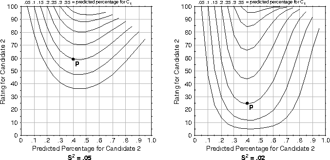
Figure: Contour plot for 3-candidate plurality election, Hoffman's
method pivot probabilities
A drawback to Hoffman's approach is that the pivot probability calculations increase in complexity with the number of candidates. For elections involving many candidates, these calculations can be quite difficult and time consuming. The reason for the increasing complexity is that Hoffman's method requires the projected outcome for all candidates to be considered in every pivot probability calculation. However, we have discovered that the only projected outcomes crucial to the pivot probability calculation are the outcomes for the candidate predicted to win and for the two candidates whose pivot probability is being computed. Furthermore, a simplifying assumption allows us to calculate pivot probabilities for N candidate elections using the predicted outcomes for just two candidates.

Figure: Predicted outcomes for candidates i and j
To calculate ![]() using our 2-D Gaussian method, we being by
plotting the predicted outcomes for i and j along an outcome line
and constructing normal distribution curves around each outcome point,
as shown in Figure
using our 2-D Gaussian method, we being by
plotting the predicted outcomes for i and j along an outcome line
and constructing normal distribution curves around each outcome point,
as shown in Figure ![]() . In ballot-by-ballot DSV it is
important that the
. In ballot-by-ballot DSV it is
important that the ![]() values used to construct the normal curves
decrease as the election progresses. We can simplify our
values used to construct the normal curves
decrease as the election progresses. We can simplify our ![]() calculation while still ensuring that
calculation while still ensuring that ![]() decreases by
substituting an average value for the numerator in the standard error
approximation presented in Equation
decreases by
substituting an average value for the numerator in the standard error
approximation presented in Equation ![]() :
:
![]()
Thus, as a ballot-by-ballot DSV election progresses, the normal curves will become increasingly narrower. However all the curves calculated for a given ballot will have the same width.
The shaded area in Figure ![]() , where the curves
intersect, represents the probability that the final outcome will
involve a tie between i and j. But not all ties are winning ties.
If our election involved only three candidates we could declare the
pivot probability to be the section of the intersection area
representing outcomes where i and j each receive between 1/3 and
1/2 of the votes. However, elections involving four or more
candidates cannot be represented this simply. To solve this problem we plot
the outcome point for the predicted winner on our outcome line and
construct a normal curve around it. As illustrated in
Figure
, where the curves
intersect, represents the probability that the final outcome will
involve a tie between i and j. But not all ties are winning ties.
If our election involved only three candidates we could declare the
pivot probability to be the section of the intersection area
representing outcomes where i and j each receive between 1/3 and
1/2 of the votes. However, elections involving four or more
candidates cannot be represented this simply. To solve this problem we plot
the outcome point for the predicted winner on our outcome line and
construct a normal curve around it. As illustrated in
Figure ![]() , the pivot probability is the intersection of
all three curves.
, the pivot probability is the intersection of
all three curves.

Figure: Geometry for calculating pivot probability using 2-D
Gaussian method
Note, that when either i or j is the predicted winner, only two
curves need be plotted. Also note, that because the curves all use
the same value of ![]() , the intersection of three curves is equal
to the intersection of the left-most and right-most curve. Thus, to
compute
, the intersection of three curves is equal
to the intersection of the left-most and right-most curve. Thus, to
compute ![]() we need only determine the area of the intersection
of the curve for the predicted winner and either i or j, whichever
is predicted to receive fewer votes.
we need only determine the area of the intersection
of the curve for the predicted winner and either i or j, whichever
is predicted to receive fewer votes.
To compute the area of the intersection we must first determine the point at which the two normal curves intersect. The point of intersection I can be calculated:
![]()
where ![]() is the predicted outcome for the predicted winner and
is the predicted outcome for the predicted winner and
![]() is the predicted outcome for either i or j, whichever
is predicted to receive fewer votes. The pivot probability
is the predicted outcome for either i or j, whichever
is predicted to receive fewer votes. The pivot probability ![]() is
then calculated:
is
then calculated:
![]()
where ![]() . Because there is no region in which ties
are guaranteed to occur, we assume the curve is infinite in both
directions. However, only half the area need be computed, as the
curve is symmetrical about the intersection point.
. Because there is no region in which ties
are guaranteed to occur, we assume the curve is infinite in both
directions. However, only half the area need be computed, as the
curve is symmetrical about the intersection point.
The above integral can be approximated using Simpson's rule or another
numerical integration technique. However, as ![]() decreases,
Simpson's rule requires increasingly more steps to converge. A more
efficient approach is to use a table of areas under the standard
normal curve or a computer function that returns the values in such a
table. In this case a change of variable must be performed to remove
decreases,
Simpson's rule requires increasingly more steps to converge. A more
efficient approach is to use a table of areas under the standard
normal curve or a computer function that returns the values in such a
table. In this case a change of variable must be performed to remove
![]() from the exponent. The pivot probability is then calculated:
from the exponent. The pivot probability is then calculated:
![]()
In our simulations we use the erf function from the C math library.
However, the erf function is not intended for use with the large upper
bound values that occur when ![]() gets very small. When our
computations using the erf function return 0, we approximate the area
as
gets very small. When our
computations using the erf function return 0, we approximate the area
as
![]()
where ![]() .
.
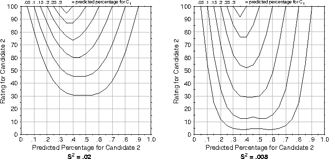
Figure: Contour plot for 3-candidate plurality election, 2-D Gaussian
method pivot probabilities
Our 2-D Gaussian method results in contour plots (shown in
Figure ![]() quite similar to those produced using
Hoffman's method. The most obvious difference between the results of
these two methods can be seen in the effects of varying
quite similar to those produced using
Hoffman's method. The most obvious difference between the results of
these two methods can be seen in the effects of varying ![]() . An
. An
![]() value approximately 0.4 times smaller than the one used in
Hoffman's method must be used in the 2-D Gaussian method to produce
similar results.
value approximately 0.4 times smaller than the one used in
Hoffman's method must be used in the 2-D Gaussian method to produce
similar results.
Another difference can be observed by comparing the upper right-hand
corners of Figures ![]() and
and ![]() . When a
voter's second-choice is predicted to win by a large margin the 2-D
Gaussian method produces pivot probabilities that will result in a
vote for the voter's first choice, regardless of
. When a
voter's second-choice is predicted to win by a large margin the 2-D
Gaussian method produces pivot probabilities that will result in a
vote for the voter's first choice, regardless of ![]() . Under the
same circumstances Hoffman's method produces pivot probabilities that
may result in a vote for the voter's second choice, depending on
. Under the
same circumstances Hoffman's method produces pivot probabilities that
may result in a vote for the voter's second choice, depending on
![]() . In this situation, the voter's first choice has practically
no chance of winning and the voter's second choice has practically no
chance of loosing. Therefore, the voter cannot influence the outcome
with his or her vote, and thus, we believe, should vote sincerely.
Hoffman's method and the 2-D Gaussian method indicate different
strategies in this situation due to the fact that for a
three-candidate race Hoffman's method indicates a higher probability
of a winning tie between third-place and first-place candidates than
between third-place and second-place candidates, while our method
indicates that the probability of a winning tie is the same for these
two pairs of candidates. Because the number of voters who must change
their votes to achieve a winning tie in each of these two situations
is identical, we believe our method is a more accurate model of pivot
probabilities involving third-place candidates.
. In this situation, the voter's first choice has practically
no chance of winning and the voter's second choice has practically no
chance of loosing. Therefore, the voter cannot influence the outcome
with his or her vote, and thus, we believe, should vote sincerely.
Hoffman's method and the 2-D Gaussian method indicate different
strategies in this situation due to the fact that for a
three-candidate race Hoffman's method indicates a higher probability
of a winning tie between third-place and first-place candidates than
between third-place and second-place candidates, while our method
indicates that the probability of a winning tie is the same for these
two pairs of candidates. Because the number of voters who must change
their votes to achieve a winning tie in each of these two situations
is identical, we believe our method is a more accurate model of pivot
probabilities involving third-place candidates.