While the expected-utility model includes a straightforward decision rule, it does not include a method for calculating pivot probabilities. Indeed this calculation appears to be anything but straightforward. Several approaches to this calculation are presented and analyzed here.
Before discussing these approaches, it is useful to examine the definition of pivot probability in more detail. As already mentioned, a voter's pivot probability for any two candidates is the probability that he or she will be decisive in making or breaking a first-place tie between those two candidates. This probability is approximately the sum of the probabilities associated with each of the possible election outcomes that involve a first-place tie between those two candidates.
The election outcome space can be represented visually as a
barycentric coordinate system --- an equilateral triangle on the
three-dimensional plane 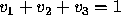 , where
  ,
,
 , and
, and  represent the percentage of votes for candidates
1, 2, and 3 respectively. Each of the triangle corners
represents one candidate. The closer an outcome point is to a
particular corner, the more votes the alternative represented by that
corner received. An outcome point in a corner of the triangle
represents a ``shut-out'' in which one alternative received all the
votes, while an outcome point in the geometrical center of the
triangle represents a three-way tie. As shown in
Figure 1, the line segments that bisect the triangle
represent two-way ties.
represent the percentage of votes for candidates
1, 2, and 3 respectively. Each of the triangle corners
represents one candidate. The closer an outcome point is to a
particular corner, the more votes the alternative represented by that
corner received. An outcome point in a corner of the triangle
represents a ``shut-out'' in which one alternative received all the
votes, while an outcome point in the geometrical center of the
triangle represents a three-way tie. As shown in
Figure 1, the line segments that bisect the triangle
represent two-way ties.
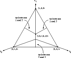
Figure 1: A Three-Dimensional View of the Barycentric Coordinate System
Because the expected-utility function depends on the ratio of the pivot probabilities rather than the actual probabilities themselves, we do not have to find a method for calculating the actual probability of reaching each point in the outcome space; rather it is sufficient to find a method of calculating relative probabilities. Thus the methods we examine here do not necessarily result in the probabilities over the entire outcome space summing to 1. This model can be extended arbitrarily; for example, when representing four-candidate elections the barycentric triangle becomes a solid tetrahedron.
One approach to calculating pivot probabilities involves making a prediction about the likely outcome of the election, plotting that outcome as a point on a barycentric coordinate system, and computing the relative distances between that outcome point and the outcome lines for each of the two-way ties. Black used this method in a model of a three-candidate plurality election in which each voter was assumed to be able to make a reasonable prediction about the election outcome based on the results of previous elections, opinion polls, or other data [3]. In our declared-strategy voting system we can determine the voters' sincere strategies from their utility information, and aggregate these strategies to determine a predicted outcome.
Black assumes that the pivot probability for any pair of candidates is
proportional to 1 minus the Euclidean distance between the line
segment  representing a first-place tie between those
candidates and the predicted outcome point A, as shown in
Figure 2. (Note that the example assumes that the
predicted outcome ranks candidate 1 in first place, 2 in second
place, and 3 in third place. If this predicted ranking does not
match the voter's preference ranking, the appropriate substitutions
must be made. For example, if the voter had the preference ranking
3 over 2 over 1, the voter's
representing a first-place tie between those
candidates and the predicted outcome point A, as shown in
Figure 2. (Note that the example assumes that the
predicted outcome ranks candidate 1 in first place, 2 in second
place, and 3 in third place. If this predicted ranking does not
match the voter's preference ranking, the appropriate substitutions
must be made. For example, if the voter had the preference ranking
3 over 2 over 1, the voter's  would refer to the
probability of a tie between candidates 2 and 3.) For
would refer to the
probability of a tie between candidates 2 and 3.) For  this distance
  is equivalent to the length of the
perpendicular line segment
is equivalent to the length of the
perpendicular line segment  from the predicted outcome
point to the first-place tie line
from the predicted outcome
point to the first-place tie line  . For
. For  the
relevant distance is
the
relevant distance is  , the length of the line
segment
, the length of the line
segment  from the predicted outcome point to the
three-way tie point D. For
from the predicted outcome point to the
three-way tie point D. For  the relevant distance
calculation depends on the percentage of votes received by the various
candidates in the predicted outcome. If the second place candidate is
predicted to receive more votes than the average of the other two
candidates (a dominant second place finish) the
the relevant distance
calculation depends on the percentage of votes received by the various
candidates in the predicted outcome. If the second place candidate is
predicted to receive more votes than the average of the other two
candidates (a dominant second place finish) the  distance is
 . Otherwise the
  distance is calculated
in the same manner as the
distance is calculated
in the same manner as the  distance. The distance calculation
for
distance. The distance calculation
for  can be expressed as:

where  and
and  .
.
 and
and  can be calculated in a
similar manner.
can be calculated in a
similar manner.
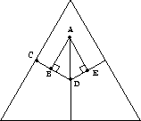
Figure 2: Distances used to calculate Black's probability estimates
One variation on Black's method involves calculating the distance d between the predicted outcome and a given point on a two way tie line. Using this technique, the pivot probability for any two candidates can be found by summing the differences 1-d for every point on the two-way tie line for those candidates. This method makes more intuitive sense than Black's method if one considers what the pivot probabilities really represent.
One problem with both Black's method and the above variation is that they assume that the probability of a tie gets linearly larger the farther away a predicted outcome point is from a two-way tie line. This uniform probability distribution, while simple, does not seem consistent with empirical evidence. For example, these methods appear never to select the strategy of voting for a second-choice candidate unless the second-choice candidate has a utility rating at least 80 percent as high as the first-choice candidate. In addition, these methods do not take into consideration the certainty of the predicted outcome point.
Hoffman [13] offers another approach which allows for the
modeling of voting schemes other than simple plurality, and assumes a
Gaussian distribution rather than a uniform distribution. As shown in
Figure 3, Hoffman specifies the region  as the
portion of the outcome triangle in which candidate i loses to
candidate j by one vote
(or less in systems that allow fractional votes).
He defines the pivot probability
as ``the probability that the election result
as the
portion of the outcome triangle in which candidate i loses to
candidate j by one vote
(or less in systems that allow fractional votes).
He defines the pivot probability
as ``the probability that the election result  lies in the region
  .'' Thus
  can be expressed
as:
can be expressed
as:
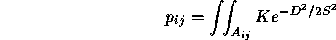
where D is the distance from the predicted outcome point to an
outcome point in  ,
,  is a measure of the uncertainty of
the prediction, and K is a constant factor. Because
is a measure of the uncertainty of
the prediction, and K is a constant factor. Because  is
only one vote wide,
is
only one vote wide,  can be approximated by using Simpson's rule
or another numerical integration technique to integrate over its face.
can be approximated by using Simpson's rule
or another numerical integration technique to integrate over its face.
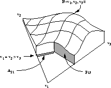
Figure 3: Hoffman's geometry for a 3-candidate election
Hoffman [13] observed that his model might break down if it were used by a large number of voters in a given election without consideration of the dynamic interaction between voters. This is a particular problem for elections in which more than one winner is selected. Hoffman suggests this problem can be overcome by introducing a probabilistic factor into the expected-utility calculation.
Hoffman's approach is appealing because it does not assume a uniform
probability distribution and because it takes into account the
uncertainty associated with the predicted outcome. Indeed this
uncertainty proves to be a significant factor in calculating a voter's
optimal strategy. Figure 4 shows the critical value
contours we have calculated for  values of
  and
and  .
Note that the y-axis shows a normalized utility rating for
.
Note that the y-axis shows a normalized utility rating for  such that
  . The figure
illustrates that the more certain the prediction, the more willing
voters should be to vote for
. The figure
illustrates that the more certain the prediction, the more willing
voters should be to vote for  rather than
  . For
example, given a predicted outcome P of
. For
example, given a predicted outcome P of  the optimal
strategy when
the optimal
strategy when  is to vote for
  if
if  .
However under the same circumstances but with
.
However under the same circumstances but with  , it is
optimal to vote for
, it is
optimal to vote for  if
if  .
.
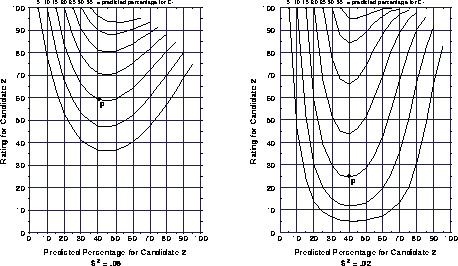
Figure 4: Critical values for 3-candidate plurality election
In our declared-strategy voting system we have several options for
obtaining  values. Normally such values are based on the size
of a sample in relation to the size of an entire population. But
because our predicted outcome point is based on polling the entire
population, our prediction derives no uncertainty from sampling error.
Rather, the uncertainty is based on not knowing how many voters will
find that their optimal strategies are not their sincere strategies.
values. Normally such values are based on the size
of a sample in relation to the size of an entire population. But
because our predicted outcome point is based on polling the entire
population, our prediction derives no uncertainty from sampling error.
Rather, the uncertainty is based on not knowing how many voters will
find that their optimal strategies are not their sincere strategies.
The simplest way to deal with uncertainty would be to select an
arbitrary value, say  . This particular value has the property
that as long as a
. This particular value has the property
that as long as a  is predicted to receive at least 5 percent of
the vote, voters will not vote for
is predicted to receive at least 5 percent of
the vote, voters will not vote for  unless
  is at least
10 percent as large as
is at least
10 percent as large as  (on a 10 point scale, a voter with
 must have
  in order to vote for
  ).
Another approach would be to
develop a formula for calculating uncertainty based on
some aggregation of the utilities submitted by the voters---perhaps
taking into account the percentage of voters for whom it might never
be optimal to voter for
).
Another approach would be to
develop a formula for calculating uncertainty based on
some aggregation of the utilities submitted by the voters---perhaps
taking into account the percentage of voters for whom it might never
be optimal to voter for  . Such a calculation is also likely to
be somewhat arbitrary, however. Still another approach would be to assign
random values to
. Such a calculation is also likely to
be somewhat arbitrary, however. Still another approach would be to assign
random values to  within a reasonable range (say .008 - .2).
Finally,
voters could select their own uncertainty
values based on their attitudes toward risk,
formulated
perhaps as a function of the ``maturity'' of the election: number of
rounds, position in the voting sequence, etc.
within a reasonable range (say .008 - .2).
Finally,
voters could select their own uncertainty
values based on their attitudes toward risk,
formulated
perhaps as a function of the ``maturity'' of the election: number of
rounds, position in the voting sequence, etc.