We wrote a declared-strategy voting simulator program to study the impact of DSV on election results. The simulator was written in C and runs on a Unix platform. Key parts of the DSV simulator source code are reproduced in Appendix B.
Our DSV simulator can simulate both ballot-by-ballot and batch mode DSV. It offers a variety of methods for calculating pivot-probabilities and uncertainty.
We implemented only one tie-breaking rule in our simulator: a bandwagon rule with persistent ties resolved randomly. Thus, all indifferent voters were assigned a strategy in which they vote for whichever candidate is winning or, in the event of a first-place tie, they select randomly from among those tied for first-place.
For each simulation, we calculated a sincere poll result in addition to a DSV result. The sincere poll result was calculated by casting a vote for the alternative rated highest by each voter. A random selection was made for voters who did not indicate a unique first choice.
We used our 2-D Gaussian method for calculating pivot probabilities in
all of the DSV simulations reported here. Other simulations using
Hoffman's method resulted in similar outcomes, but with less strategic
voting (probably due to differing affects of ![]() in the two methods).
in the two methods).
Batch DSV simulations were run with two arbitrary values of ![]() :
.001 (which we shall hereafter refer to as ``small
:
.001 (which we shall hereafter refer to as ``small ![]() '') and
.05 (which we shall hereafter refer to as ``large
'') and
.05 (which we shall hereafter refer to as ``large ![]() ''). Batch
simulations were run for as many rounds as necessary for an
equilibrium to be reached. An equilibrium was reached in all
simulations without the need for an arbitrary cut-off.
''). Batch
simulations were run for as many rounds as necessary for an
equilibrium to be reached. An equilibrium was reached in all
simulations without the need for an arbitrary cut-off.
Ballot-by-ballot simulations were run 1000 times on each data set.
The ballots in each set were shuffled randomly before each run. The
results reported are the average results over all the runs. The
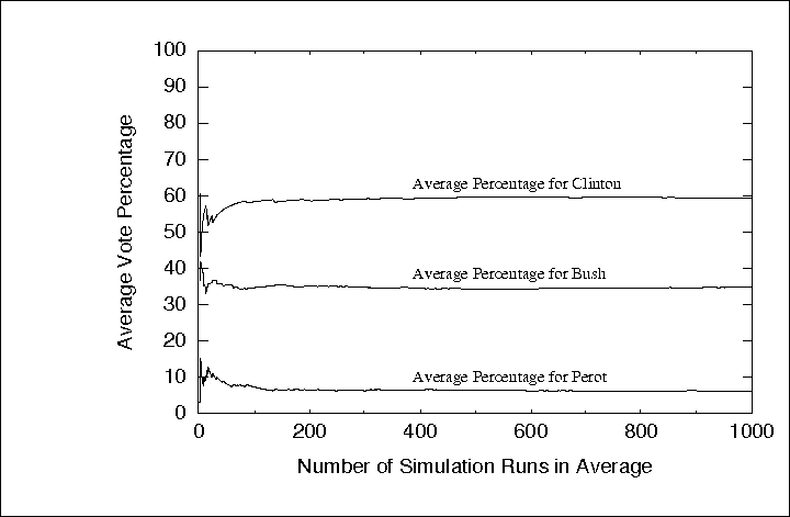
running average for most of our simulations became fairly stable
(varying by less than 1%) after the results of a few hundred
simulations were included in the average. For example,
Figure ![]() shows the running average for
ballot-by-ballot DSV simulations using data from the 1992 National
Election Study (to be discussed in Section
shows the running average for
ballot-by-ballot DSV simulations using data from the 1992 National
Election Study (to be discussed in Section ![]() ).
).

Figure: Running average for ballot-by-ballot DSV simulation of 1992
US Presidential election
We simulated the selection of topics for a university lecture series using data collected from 162 respondents who answered question 2 of our survey. The respondents were asked to rate their interest in each of ten possible lecture topics (anthropology, gender issues, health and medicine, history, journalism/media, literature, politics, race relations, science, and sports) on a scale of 0 to 10. As shown in the table below, the sincere poll indicated that science was the most popular topic with 20.4% of the vote, followed closely by sports with 19.1%. Health and politics each received over 10% of the vote as well. Batch DSV also resulted in a victory for science, followed by sports, health, and politics. A decision-maker who could select several lecture topics for inclusion in the lecture schedule would be wise to select these four.

The ballot-by-ballot DSV results indicated that science and health were significantly more popular than sports or politics when preferences beyond each voter's first choice were considered. Science averaged 33.9%, winning the ballot-by-ballot DSV election 47% of the time. Health averaged 30.0%, winning 46% of the time. Sports averaged 21.4%, winning 7% of the time, and politics averaged 9.4%, winning less than 1% of the time. An analysis of the individual ballot-by-ballot simulations indicated that in the simulations where science won, health received a low percentage of votes, and in the simulations where health won, science received a low percentage of votes. This indicates that the respondents who were interested in science were likely to be almost as interested in health, and visa versa (thus both groups could be satisfied by the selection of either lecture topic). This observation could be made because DSV allowed those who preferred health and science to pile on to whichever of these topics was more likely to win rather than splitting their votes. Thus DSV is helpful to both the survey respondents and the decision-maker in this situation.
The batch DSV results are less useful to a decision-maker. When
![]() is very small, batch DSV tells us only that science is the
most popular topic. When
is very small, batch DSV tells us only that science is the
most popular topic. When ![]() is large, batch DSV shows us that
science is a more popular second choice than the other leading
contenders.
is large, batch DSV shows us that
science is a more popular second choice than the other leading
contenders.
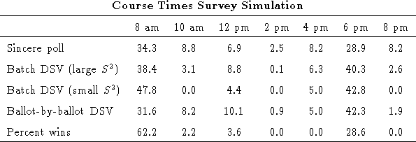
We simulated the selection of a course time using data from the 159 respondents who answered question 3 of our survey. The respondents were asked to rate their interest in taking a course at each of seven possible times of day (8:00 am, 10:00 am, 12:00 pm, 2:00 pm, 4:00 pm, and 8:00 pm) on a scale of 0 to 10. As shown in the table below, the sincere poll indicated that 8:00 am was the most popular time, followed closely by 6:00 pm. However ballot-by-ballot DSV showed that 6:00 pm would actually please more people. Under ballot-by-ballot DSV, 6:00 pm won with an average of 42.3%, while 8:00 am came in second with an average of 31.6%. Indeed an analysis of respondents' ratings for just these two time slots indicates that 66% preferred 6:00 pm to 8:00 am. It is also useful to note that while 8:00 am actually won more ballot-by-ballot DSV elections than 6:00 pm, 6:00 pm came in a close second in most of the elections in which 8:00 am won, while 8:00 am was nearly shut out in most of the elections in which 6 pm won. This is due to the fact that most of the respondents who preferred 6 pm found most other times completely unacceptable, while the respondents who preferred 8 am found other times acceptable as well.

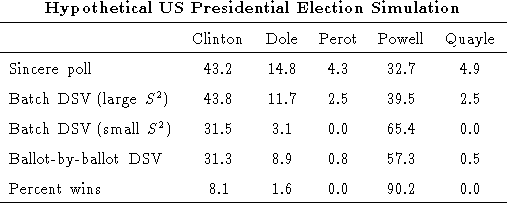
We simulated a hypothetical US Presidential election using data from
the 164 respondents who answered question 6 of our survey. The
respondents were asked to rate their approval for each of five
hypothetical Presidential candidates (Bill Clinton, Bob Dole, Ross
Perot, Colin Powell, and Dan Quayle) on a scale of 0 to 10. As shown
in the table below, the sincere poll elected Clinton, with Powell in
second place. However simulations using ballot-by-ballot DSV and
batch DSV with small ![]() values elected Powell with Clinton in
second place. This is due to the fact that many Dole, Perot, and
Quayle supporters also supported Powell. The ballot-by-ballot
simulations were fairly stable for this election, electing Powell
90.2% of the time.
values elected Powell with Clinton in
second place. This is due to the fact that many Dole, Perot, and
Quayle supporters also supported Powell. The ballot-by-ballot
simulations were fairly stable for this election, electing Powell
90.2% of the time.

Further examination of the ballots revealed that over a quarter of the respondents did not have a unique first choice. A sincere poll conducted without these respondents elected Powell with 39.5% of the vote. Ballot-by-ballot DSV without these respondents was even more stable than with all respondents, electing Powell 96.9% of the time. This increase in stability highlights the fact that much of ballot-by-ballot DSV's instability is due to indifferent voters. It might be argued that if voters are indifferent -- either individually or collectively -- then it is appropriate for a voting system to return unstable results. Indeed stable results essentially misrepresent the winner as being more preferred by the electorate when in fact he or she is equally preferred to one or more other candidates.
One of the most well-documented examples of the use of decision
analysis to facilitate real-life group decision-making in the
literature is Dyer and Miles' account of the selection of trajectories
for NASA's 1977 Mariner Jupiter/Saturn project [42]. About
80 scientists divided into ten science teams were asked to select a
single pair of spacecraft trajectories that would provide the best
data collection opportunities for all teams. To facilitate this
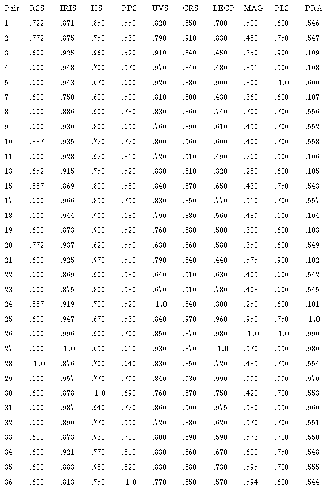
decision the science teams were asked to each provide their ordinal
and cardinal preferences for 32 pairs of proposed trajectories
(numbered consecutively from 1 to 36 with numbers 6, 12, 14, and 16
deleted). These preferences (shown in Figure ![]() with
the science team names abbreviated at the top of each column) were
then aggregated using several collective choice rules -- some which
used ordinal rankings and some which used cardinal utilities -- and
the results were presented to the scientists. Depending on the
collective choice rule used, pair 26, 29, or 31 appeared to be the
best collective choice. (These pairs were ranked in the top three by
every collective choice rule considered.) After some discussion the
scientists selected pair 26 and asked that it be modified slightly.
with
the science team names abbreviated at the top of each column) were
then aggregated using several collective choice rules -- some which
used ordinal rankings and some which used cardinal utilities -- and
the results were presented to the scientists. Depending on the
collective choice rule used, pair 26, 29, or 31 appeared to be the
best collective choice. (These pairs were ranked in the top three by
every collective choice rule considered.) After some discussion the
scientists selected pair 26 and asked that it be modified slightly.

Figure: Mariner science team cardinal utility values
We used the science teams' cardinal utilities to simulate the trajectory pair selection under DSV. This simulation was different from the others we performed in that it involved a small number of voters and a large number of alternatives. In this type of voting situation ballot-by-ballot DSV is highly dependent on chance.
In 1000 ballot-by-ballot DSV simulations, pair 27 averaged 23.7% and
was selected 40.3% of the time. Pair 26 averaged 34.5% and was
selected 20.3% of the time. Pair 25 averaged 22.8% and was selected
23.2% of the time. The only other pair to be selected was pair 5,
which was selected less than 1% of the time. Batch DSV with small
![]() values selected pair 26 with 50% of the vote. Due to the
small number of voters and large number of alternatives, no strategic
voting occurred under batch DSV with large
values selected pair 26 with 50% of the vote. Due to the
small number of voters and large number of alternatives, no strategic
voting occurred under batch DSV with large ![]() values.
values.
The top three pairs selected by our simulations (25, 26, and 27) were ranked in the top 9 by every collective choice rule used in Dyer and Miles' study. Pair 26 was ranked in the top 3 by every rule.
Our DSV simulations never selected pairs 29 or 31, which were in the set of pairs selected by the other collective choice rules. This is due to the fact that neither of these pairs was ranked first by any science team. This observation highlights the fact that DSV systems that use the plurality rule will never select an alternative that is widely preferred as a second choice unless it also makes a strong showing as a first choice. This is not a property of DSV systems in general, rather it is a property of plurality rule systems. A DSV system that used an approval voting rule would not have this property. In a case such as this where selecting a good compromise alternative is a high priority, DSV with approval voting might prove more useful than DSV with plurality rule.
Another interesting observation about DSV in this situation is that it
does not take into account the fact that some popular alternatives may
be strongly disliked by a minority. For example, choice 27 is ranked
first by ballot-by-ballot DSV despite being ranked ![]() by one of
the science teams. In the collective-choice rules that take into
account each voter's entire preference order, a low ranking such as
this would hurt a popular alternative, acting effectively as a
negative vote. As with all single-vote systems, DSV systems do not
factor in low rankings. However, unlike plurality-rule elections, in
elections where DSV is used, the data is available for analysts to
determine whether the selected alternative was strongly disliked by a
minority.
by one of
the science teams. In the collective-choice rules that take into
account each voter's entire preference order, a low ranking such as
this would hurt a popular alternative, acting effectively as a
negative vote. As with all single-vote systems, DSV systems do not
factor in low rankings. However, unlike plurality-rule elections, in
elections where DSV is used, the data is available for analysts to
determine whether the selected alternative was strongly disliked by a
minority.